The DynamoDB Adjacency List Pattern

A graph is just nodes and edges, and the adjacency list pattern stores both as plain items in one table. Each edge becomes a row whose is the source node and whose sort key is the target. Querying a partition lists every neighbor — the DynamoDB stand-in for a JOIN on a join table.

What is the DynamoDB adjacency list pattern?

The adjacency list pattern models a graph as edge items in one table: each relationship (A follows B) is a row keyed by source on the and target on the sort key. Querying a partition lists every neighbor, and a flipped inverts the relationship — no joins, no scans, both directions in a single query.

Edges are items. Model each relationship (user A follows user B) as its own item keyed by source on the partition key, target on the sort key.
One direction is free; the other needs a . The base table answers "who does A follow?". A flipped index answers "who follows A?".
No joins, no scans. Both directions are a single Query against a known partition — never a full-table Scan.
It's the many-to-many primitive. Follows, memberships, likes, friendships — any graph where one entity connects to many others fits this shape.

Frame it as access patterns

Coming from SQL, a follow graph is a join table: follows(follower_id, followee_id). To list someone's followers you index one column; to list who they follow you index the other. DynamoDB has no joins, so you design the keys to serve each read directly.

Write down the reads first. For a social follow graph:

Who does user A follow? (their following list)
Who follows user A? (their followers list)
Does A follow B? (a single point lookup)

The keys exist only to answer that list. Get them right and every read is one Query or GetItem.

Model edges as items

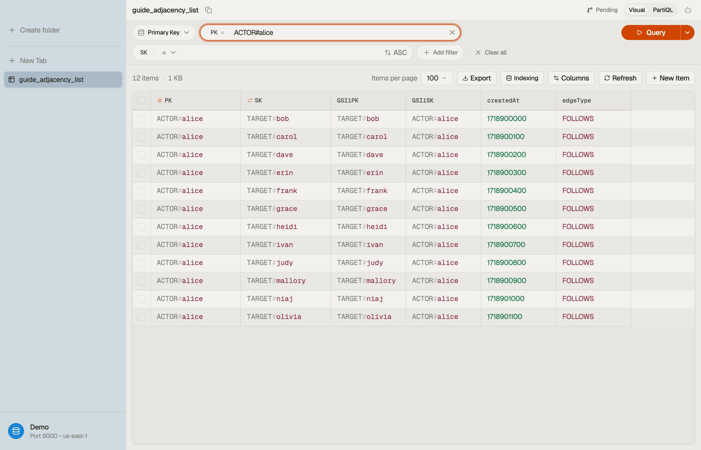
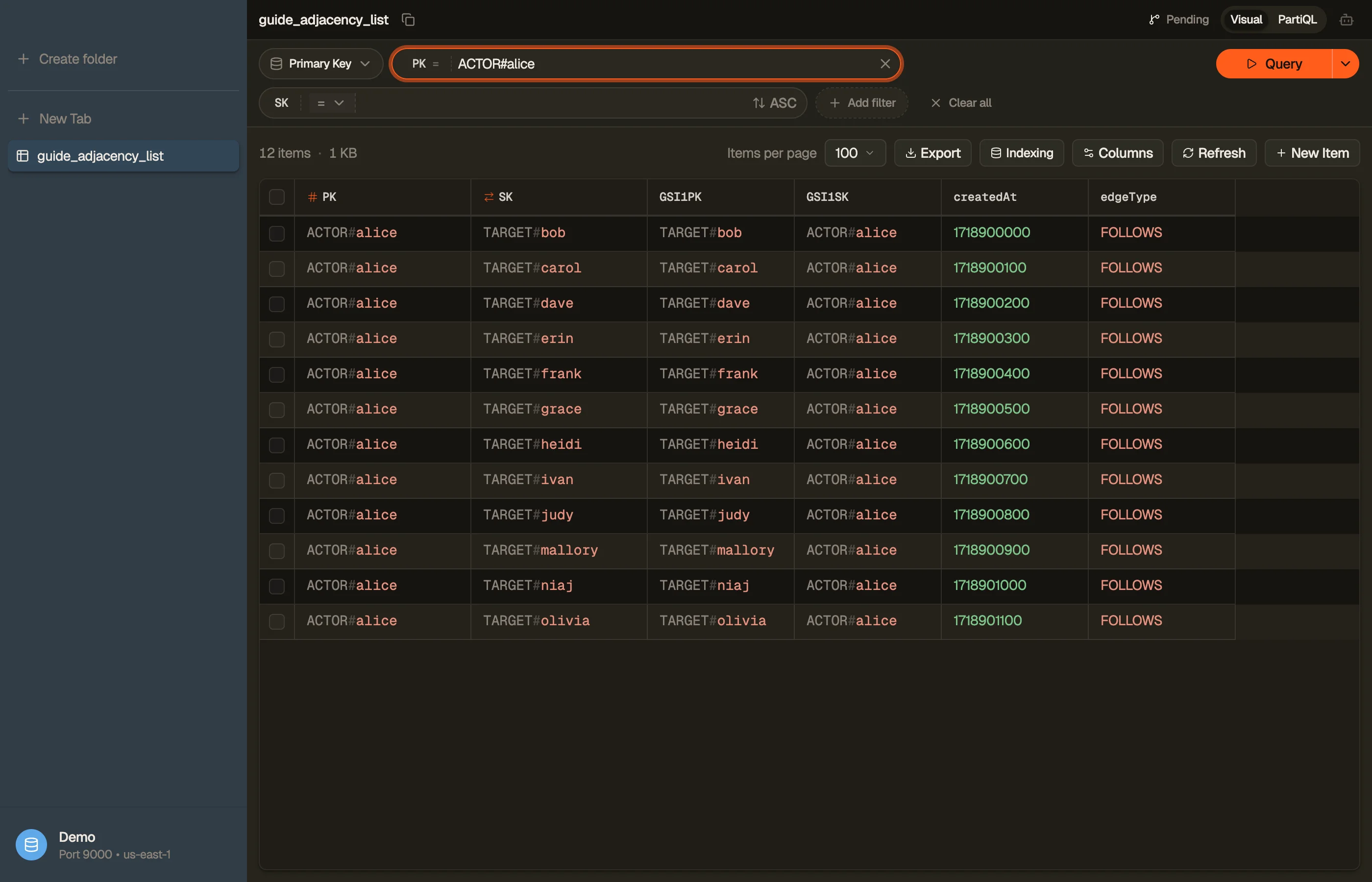
Use generic key names so the table can hold more than one entity type, and encode the node type in the value. A follow edge looks like this:

PK	SK	createdAt	edgeType
ACTOR#alice	TARGET#bob	1718900000	FOLLOWS
ACTOR#alice	TARGET#carol	1718900100	FOLLOWS
ACTOR#dave	TARGET#bob	1718900200	FOLLOWS

PK = ACTOR#alice is the source of the edge; SK = TARGET#bob is who she follows. One Query PK = "ACTOR#alice" returns every account Alice follows in a single billed read — her entire following list, no joins.

Each edge is written once, in the direction "who I follow". The reverse direction ("who follows me") is the part the base table can't answer — yet.

Traverse the other direction with a GSI

The base table is keyed source-first, so it can't answer "who follows Bob?" without scanning. Add a global secondary index that flips the keys: project the target onto the index partition key and the source onto the index sort key.

GSI1PK	GSI1SK	(base item)
TARGET#bob	ACTOR#alice	ACTOR#alice → TARGET#bob
TARGET#bob	ACTOR#dave	ACTOR#dave	→ TARGET#bob
TARGET#carol	ACTOR#alice	ACTOR#alice → TARGET#carol

Now Query GSI1 WHERE GSI1PK = "TARGET#bob" lists everyone who follows Bob — alice and dave — in one read. The same edge item serves both directions: the base table is following, the index is followers. You write each edge once and get both queries for free.

This is exactly the pattern AWS documents in its DynamoDB best-practices guide for modeling many-to-many relationships and graph data — store edges as items, then use a GSI to invert the relationship.

Check a single edge cheaply

"Does Alice follow Bob?" doesn't need either list. Because the edge is keyed PK = ACTOR#alice, SK = TARGET#bob, it's a direct GetItem — the cheapest read DynamoDB offers, no Query, no index.

To write the follow idempotently and avoid double-counting, guard the PutItem with a condition that the edge doesn't already exist:

attribute_not_exists(PK)

You can assemble that condition — and the marshalled key values — with the DynamoDB expression builder instead of hand-writing the ConditionExpression and ExpressionAttributeValues.

Do it in DynoTable

When you browse the table, the edges for one actor stack under a single partition key as one , and switching to the GSI view shows the inverted followers list — the two halves of the relationship side by side.

DynoTable showing one actor's follow-edge items under a single partition, with the GSI key attributes visible as columns.

Pitfalls

The celebrity partition. A user with millions of followers concentrates every follower edge under one GSI1PK = TARGET#<star> partition. Reads of that collection are paginated and can run hot. For fan-out-heavy graphs, shard the hot key (e.g. TARGET#bob#0..N) or denormalize counts so you don't re-read the whole list.

Storing counts on the edge. A follower count isn't an edge — don't derive it by reading and counting the whole partition on every profile view. Maintain a counter attribute on the user item and update it transactionally with the edge.

Forgetting the reverse write isn't needed here. A classic adjacency-list variant writes the edge twice with ids swapped. With a flip-key GSI you write it once and let the index materialize the reverse — fewer writes, no drift between the two copies.

Next steps

The adjacency list is the relationship building block of single-table design; the inverting index is a GSI, not an LSI, because the partition key changes. And every read here is a Query or GetItem on a known key — never the Scan footgun.

Build the condition and key expressions with the DynamoDB expression builder, and download DynoTable to model a follow graph against your own table and watch both directions resolve in one read.