How we built a local SQL engine for DynamoDB

DynamoDB can export a 100 GB table, but it cannot aggregate one. It has no JOIN and no GROUP BY. Its only exact count is the per-page Count that a Query or Scan returns with Select=COUNT, which you add up yourself.

PartiQL, AWS's own SQL-like interface, does not add them. So teams write the same throwaway script again and again: paginate a Scan, fold rows into a map, print the answer, delete the script.

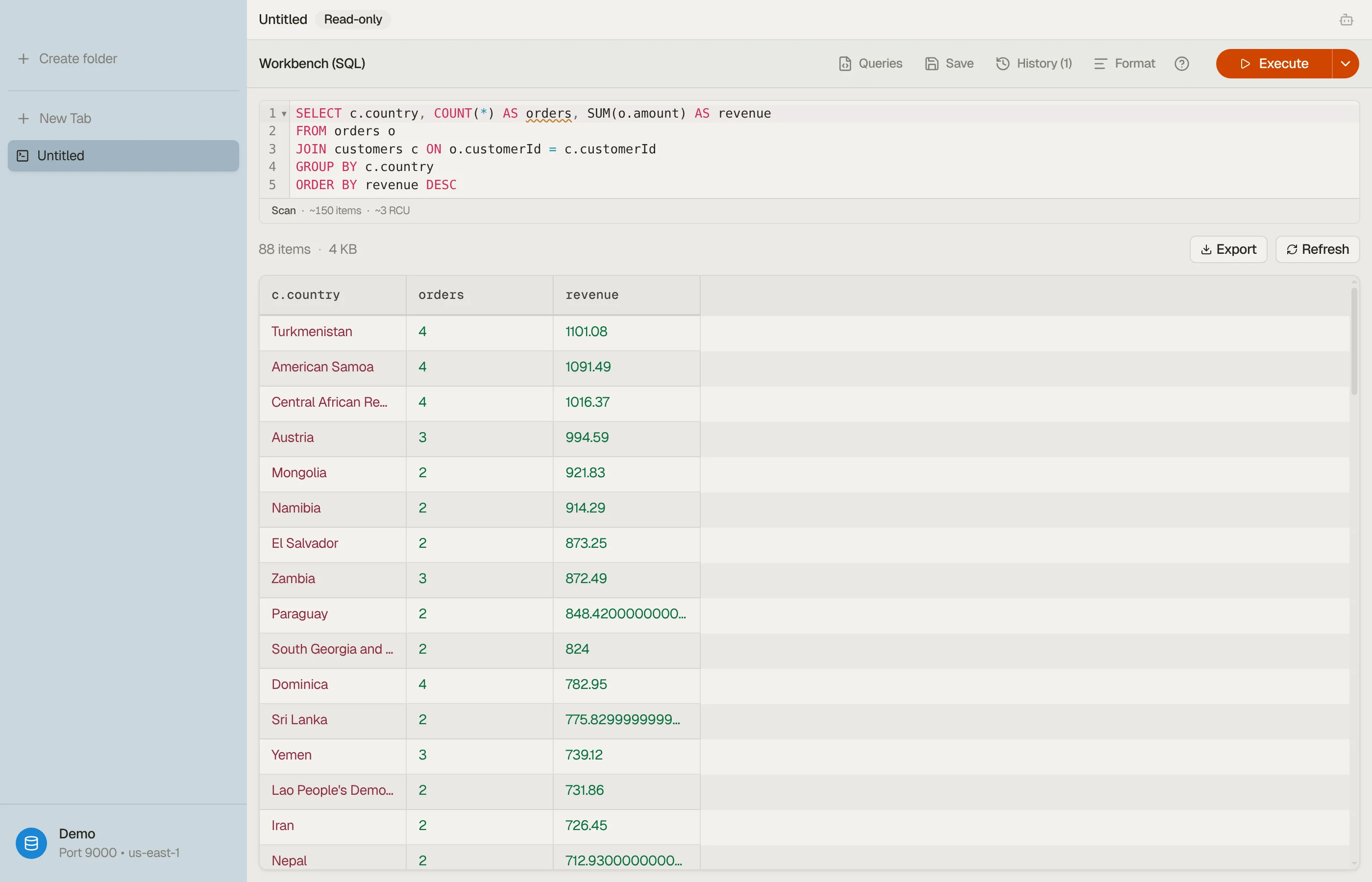
DynoTable's Workbench replaces that script. It is a tab where you write one SELECT with multi-table JOIN … ON, WHERE, GROUP BY, HAVING, DISTINCT, CASE and aggregates.

This post covers how it works, the first compiler that returned wrong answers without an error, and why we later replaced the engine's memory model.

We compile SQL onto an engine that already exists

The core decision was to not write a relational executor. DynamoDB pages stream into an embedded SQLite database, and SQLite does the relational work. Our code is the compiler between your SQL and that engine.

Each DynamoDB item lands in SQLite as its raw typed envelope, such as {"platform": {"S": "ios"}}, in a single column. A small user-defined function unwraps attributes at query time.

So your SELECT platform compiles to a call to that function. The function catches its own JSON parse errors and returns NULL for that row.

Without the catch, the SQLite binding turns one malformed row's error into an abort of the whole statement.

A Workbench tab runs SQL within DynamoDB's access-pattern rules. A JOIN must land on the partition key of a table that has no sort key, or on a GSI partition key.

The engine resolves each join by key lookup and never scans the joined table. A join on a non-key attribute gets a compile error. Fixing it is a data-modeling question.

Our first compiler returned wrong answers without an error

The first version used a popular off-the-shelf SQL parser. Within about a week, four correctness bugs piled up, and the parser blocked the fix.

Two of them lived in the emitter. That is the part of the compiler that turns each parsed node back into SQL for the local engine.

• SELECT DISTINCT was dropped without a warning. The parser accepted it and the emitter ignored it, so every duplicate row came back. One user's bug report read: "shows a table of all the values, not counters."
• Any unhandled syntax became the literal SQL NULL. For CASE, CAST and scalar subqueries, the emitter fell back to return 'NULL'. Queries ran, returned wrong answers and raised no error.
• Identifier case did not behave like SQL. SELECT PLATFORM FROM t returned nulls when the attribute was platform. Standard SQL treats unquoted names as case-insensitive.
• Autocomplete missed matching names. Typing a name in a different case found nothing, and suggestions for quoted names did not always appear.

We picked the parser that keeps the quotes

The replacement, sql-parser-cst, was the only parser we evaluated whose tree keeps both the raw text and the normalized name of every identifier. With both, the compiler can tell platform from "PLATFORM".

That one distinction gives a single grammar proper ANSI semantics. Unquoted identifiers resolve case-insensitively. Quoted identifiers are the case-sensitive escape hatch, as in Postgres.

Without it, case-insensitive lookup and correct autocomplete could not both be right. A strict match drops rows. A fully case-insensitive match removes your way to pick platform over Platform when an item has both.

The parser also attaches a source range to every node, so a diagnostic underlines the exact construct that failed.

We replaced the return 'NULL' fallback with a fixed rule. Anything the emitter does not support raises an error on that node's range. A window function gets this one:

Unsupported expression: window function. Supported: column refs, literals, arithmetic, comparison, AND/OR/NOT, IN, BETWEEN, IS NULL, LIKE, CASE, CAST, function calls, aggregates. Not yet: window functions, scalar subqueries, set operations, CTEs.

The message lists what the Workbench does support, so you can rewrite the query without guessing.

sql-parser-cst is pre-1.0. We pin the exact version and upgrade it only by hand, with the test suite as the gate.

We rejected five alternatives. Patching the old parser needed a second tokenizer to recover quote information, so every input would be parsed twice.

Reusing the editor's own syntax tree failed because that tree is token-level, with no clause structure for a compiler to walk.

Writing our own parser meant most of a SQLite parser and maintenance with no end. Waiting for sql-parser-cst 1.0 left four correctness bugs in front of users.

Restricting the Workbench to the SQL the old parser handled would have banned CASE, CAST and DISTINCT, which SQL users expect to work.

One warning deliberately does not block the query. A filter can name an attribute whose case the schema cannot confirm, because DynamoDB declares only key attributes and its server-side filters are case-sensitive.

That filter gets a warning, and warnings never stop a query from running. Our validator work taught the same lesson. A gate that rejects the most common valid query does more harm than no gate.

Buffering in memory failed on big tables or answered from part of them

The first aggregation engine buffered scanned rows into an in-memory SQLite database. The AI agent's SQL tool capped it at 64 MB or 100,000 rows, and its transform tool at 250 MB. Hitting a cap failed the query.

The Workbench tab had no cap. It aggregated the pages loaded so far, and loading every page of a large table could run the app out of memory.

For the redesign, we asked what the throwaway script would do. A competent script streams and folds each page into a running total, so its memory stays bounded.

A GROUP BY over part of a table gives a wrong answer, and a ranking built from it puts the wrong rows first. Our own AI demo once presented a partial "top spenders" ranking as fact.

A planner streams or stores each query

The Workbench tab now stores its pages in a disk-backed SQLite file, so a run to the end no longer has to fit in memory.

The SQL tool that the AI agent and MCP clients call goes further. It works the way the script does, then adds what the script skips. A planner reads each query first and picks one of two paths:

• Fold as it streams. Plain COUNT, SUM, AVG, MIN and MAX over one table, with every projected column in the GROUP BY. DynoTable folds each page into a running total.
• Store, then query. Sorts, key-bounded joins and the other queries the planner can model land in a disk-backed SQLite file. Free disk space sets the limit.

When the planner cannot model a query, the tool falls back to an ad-hoc route. It streams each referenced table into a SQLite file and runs the SQL there.

So a join on a non-key attribute works for the agent and over MCP, where a Workbench tab rejects it. The price is a full scan of every table in the query.

For the in-app agent, table size never blocks the fold path; a bigger table only takes longer.

The fold path is deliberately narrow. A WHERE, HAVING, ORDER BY or LIMIT, a join, or a column missing from the GROUP BY sends the query to the store path.

The fold applies none of those clauses. A fold that skipped one and still reported an exact result would be the confident wrong answer this planner exists to prevent.

Exactness is part of the result. In a Workbench tab, an aggregate carries a partial badge while pages stream, and the badge drops only when the scan has finished.

On the streaming path, integer sums stay exact past 2⁵³ because the engine stores them as 64-bit integers. A fractional sum above 2⁵³ marks itself partial instead of rounding without a word.

On the store path, any value past 2⁵³ marks the result partial.

Big scans need consent. In the app, running a single-table tab to the end over a table of more than 5 million items or 1 GiB asks you first. That includes a tab the AI agent opens.

MCP callers have no dialog, so they get a scan budget instead: 50 million items, 50 GiB or 30 minutes. A cancelled request stops the scan.

The result a model reads, in the app or over MCP, is trimmed on purpose. It carries exactness and the count of items scanned, but no size estimate. That estimate comes from table metadata that can be hours old.

A model given a stale guess narrates it as fact, so we leave the guess out.

For a one-off aggregate, a live Scan is the cheaper path. In us-east-1, a full Scan with eventually consistent on-demand reads costs about one sixth of a DynamoDB export to S3.

With strongly consistent reads, the Scan costs about a third of the export. Export also requires point-in-time recovery on the table.

So a live Scan is the default, and export plus Athena is the recommendation for repeated heavy analytics. The pricing calculator estimates your monthly read and write cost.

SQL in the Workbench cannot write to your table

The SQL that reaches the local engine must be one read-only SELECT. Anything else is refused before it runs and treated as a compiler bug, because the compiler should never produce it.

The engine also runs with extension loading and other risky built-ins turned off. Workbench SQL has no path that writes to DynamoDB. Edits you make in the grid and item editor are staged first, except a bulk direct run.

What transfers if you're building one

• Compile onto an engine that already exists. Your bugs will live in the seams: identifier case, type envelopes, corrupt rows.
• Demand quote information from your parser. If it cannot tell name from "NAME", you cannot implement SQL's case rules.
• Make unhandled syntax a loud error. A silent NULL default is how confident wrong answers ship.
• Measure your design against the throwaway script your user would write. If the script streams and you buffer, change the design.
• Label partial aggregates as partial. Users read an unlabeled number as the answer.

The Workbench docs cover the day-to-day feature set. SQL for DynamoDB maps what works across the whole ecosystem.

To try it, download DynoTable, open a Workbench tab with ⌘⌥B and run a JOIN against a database that does not have one.